Understanding Bayes · pattern recognition study

From observations
to probabilities.

What makes a measurement belong to one class rather than another? A study of Bayesian classification, built through Gaussian kernels, covariance matrices, and a small dataset of flowers.

Iris datasetParzen windowsQDF & MQDFPython · NumPy

The starting point

Three species.
Overlapping evidence.

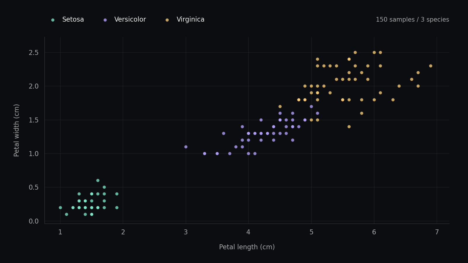
Scatter plot of the 150 bundled Iris observations. Setosa clusters at small petal lengths and widths; Versicolor and Virginica overlap around petal lengths of 4.5 to 5.5 centimeters.
01 / Observe

Two of the four measured features, plotted from the repository’s Iris data. Every observation is included; identical coordinates overlap.

How should a class
explain an observation?

This project began as an INT304 pattern-recognition assignment on non-parametric classifiers and discriminant functions. The core question is practical: given a flower’s measurements, which of three species best explains them?

Bayes’ rule connects the prior probability of a class to the likelihood of seeing an observation within it. Comparing the resulting posterior probabilities gives a classification decision.

Bayes’ rule
P(ω | x) = P(ω) p(x | ω)p(x)

For a fixed observation, the denominator is shared by every class. With equal class priors, the comparison reduces to the class likelihoods. The interesting work happens inside that likelihood: how do we estimate it from examples?

150Iris observations
4measured features
3flower species

Let every observation
contribute a little evidence.

A Parzen-window estimate places a small kernel around each training example and adds their contributions. Here, the kernel is Gaussian: nearby observations contribute more, and distant ones contribute less.

Gaussian Parzen window
p̂(x | ω) = 1nω hd ∑ φd((x − xi) / h)

The sum runs over examples in class ω; nω is their count, d is the number of features, and φd is the standard d-dimensional Gaussian density. The bandwidth h controls how much each example spreads out.

Small windows preserve local detail. Wide windows smooth it away. The decision changes with the density we choose to see.
Change the window.
Watch the evidence move.

Adjust the bandwidth, then move the observation through the three distributions. Where two curves overlap, the model’s preference becomes less clear.

Enable JavaScript to explore the distributions. In the default example, a 4.70 cm petal with h = 0.35 gives approximately 0.0% Setosa, 66.3% Versicolor, and 33.7% Virginica.

An illustration built for this page using all 150 bundled observations and only petal length. It demonstrates a one-dimensional Gaussian KDE with equal priors; the coursework evaluates classifiers using all four features and held-out folds.

Another route:
describe the shape of a class.

A quadratic discriminant takes a different approach. Each class is described by a mean and covariance matrix. A point is judged by how far it sits from that mean, taking the class’s spread and correlations into account.

QDF / equal priors · lower cost wins
g(x) = (x − μ)T Σ−1 (x − μ) + log |Σ|

Small estimated variances can make a covariance-based decision sensitive to limited data. The modified discriminants explore two ways of controlling that sensitivity.

G₀ / QDF

Use the full covariance

Model the class with its estimated mean and covariance. Every direction contributes to the quadratic distance.

G₁ / MQDF

Give every direction a floor

Add h²I to the covariance. Each eigenvalue becomes λ + h², reducing the influence of directions with very small estimated variance.

Σ → Σ + h²I
G₂ / MQDF

Keep the leading directions

Retain k principal directions and use a common variance h² for the rest. The model can vary how much covariance detail it preserves.

λ₁, …, λₖ, h², …, h²

These describe the intended mathematical models. The repository preserves the original coursework implementation; its historical results below are presented as reported.

One dataset.
Five held-out views.

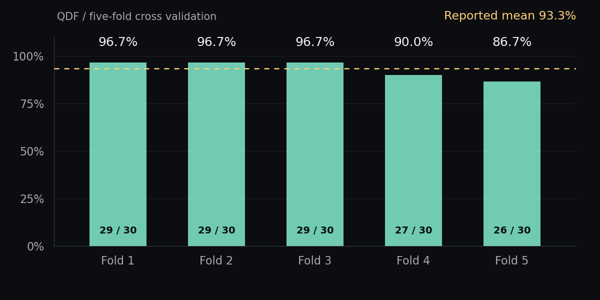
The study shuffles the Iris data with a fixed seed of 17, then uses five folds: 120 training samples and 30 test samples per fold. The original report records the following results for the baseline quadratic discriminant.

Historical QDF results: folds one, two and three each classified 29 of 30 samples correctly, or 96.7 percent; fold four 27 of 30, or 90 percent; fold five 26 of 30, or 86.7 percent. Reported mean 93.3 percent.
Redrawn from the five fold scores in the original report. These are historical results, not a new benchmark run.

The other experiments sweep h for Parzen windows and MQDF1, then vary h and k for MQDF2. Their plots make parameter sensitivity visible: changing the model’s assumptions can change the decisions even when the dataset stays the same.

The parameter sweeps.

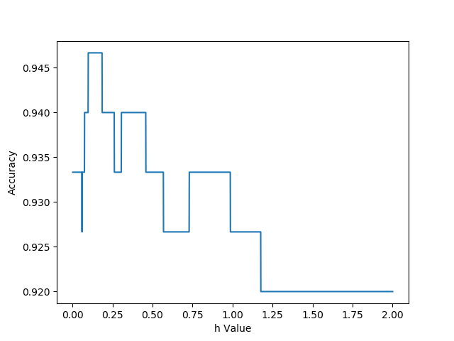
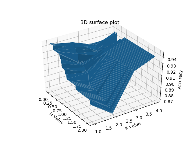
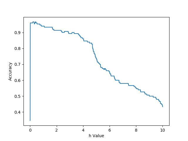
The three original figures, preserved from the repository. Open a figure to inspect its axes and parameter-sweep results.

Original Parzen-window accuracy plot across bandwidth values
01 / Parzen

Choosing a window

Classification accuracy as the Gaussian bandwidth h changes.

Original MQDF1 accuracy plot across regularization values
02 / MQDF1

Stabilizing the estimate

The effect of covariance regularization on mean five-fold accuracy.

Original three-dimensional MQDF2 plot of accuracy against h and k
03 / MQDF2

Keeping fewer directions

A joint view of h, the retained dimension k, and accuracy.

Make the assumptions
visible in the code.

The classifiers are written directly with NumPy operations, so density estimates, eigenvalues, and discriminant costs remain visible. pandas handles data loading, Matplotlib draws the experiments, and scikit-learn supplies the fold splitter.

The value of this exercise is the connection between a formula and a decision: how bandwidth sets the scale of evidence, how covariance describes a class, and how regularization changes the shape we are willing to trust.

Understanding by
building the steps.

A learning project about what Bayesian classification asks of the data, and what changes when the density model changes. The source, report, and original figures remain together as a record of that exploration.